Grad-CAM は、畳み込みニューラルネットワークの最後の畳み込み層により抽出された特徴量に着目して、機械学習が画像のどの部分を見ているのかを可視化する方法である。このページでは、PyTorch で構築した畳み込みニューラルネットワークに Grad-CAM を適用して、画像の判断根拠部分の可視化を行う方法を紹介する。
Grad-CAM は、最後の畳み込み層の出力を使用して計算する。そこで、訓練済みのモデルに画像を代入して、モデルの各層を少しずつ実行していき、最後の畳み込み層の結果をいったん変数に保存して、それに対して Grad-CAM を計算する。幸いにも PyTorch で構築されたモデルは、レイヤーの順序が明確で、しかも、一部のレイヤーがまとめられてモジュール化されているので、非常にとり扱いやすい。以下に、VGG16 および ResNet18 のモデル(アーキテクチャ)に Grad-CAM を適用する方法を示す。
VGG16
PyTorch で構築された(あるいは転移学習を行ったあとの) VGG16 のモデルに Grad-CAM を適用する方法を示す。モデルの訓練から Grad-CAM までの流れを示した全コードは ![]() を参照のこと。ここでは、訓練済みのモデルがすでに用意されて、
を参照のこと。ここでは、訓練済みのモデルがすでに用意されて、net_ft という変数に保存されているものとする。まず、net_ft のアーキテクチャを出力して、各層の構造を確認する。
print(net_ft)
# VGG(
#   (features): Sequential(
#     (0): Conv2d(3, 64, kernel_size=(3, 3), stride=(1, 1), padding=(1, 1))
#     (1): ReLU(inplace=True)
#     (2): Conv2d(64, 64, kernel_size=(3, 3), stride=(1, 1), padding=(1, 1))
#     (3): ReLU(inplace=True)
#     (4): MaxPool2d(kernel_size=2, stride=2, padding=0, dilation=1, ceil_mode=False)
#     (5): Conv2d(64, 128, kernel_size=(3, 3), stride=(1, 1), padding=(1, 1))
#     (6): ReLU(inplace=True)
#     (7): Conv2d(128, 128, kernel_size=(3, 3), stride=(1, 1), padding=(1, 1))
#     (8): ReLU(inplace=True)
#     (9): MaxPool2d(kernel_size=2, stride=2, padding=0, dilation=1, ceil_mode=False)
#     (10): Conv2d(128, 256, kernel_size=(3, 3), stride=(1, 1), padding=(1, 1))
#     (11): ReLU(inplace=True)
#     (12): Conv2d(256, 256, kernel_size=(3, 3), stride=(1, 1), padding=(1, 1))
#     (13): ReLU(inplace=True)
#     (14): Conv2d(256, 256, kernel_size=(3, 3), stride=(1, 1), padding=(1, 1))
#     (15): ReLU(inplace=True)
#     (16): MaxPool2d(kernel_size=2, stride=2, padding=0, dilation=1, ceil_mode=False)
#     (17): Conv2d(256, 512, kernel_size=(3, 3), stride=(1, 1), padding=(1, 1))
#     (18): ReLU(inplace=True)
#     (19): Conv2d(512, 512, kernel_size=(3, 3), stride=(1, 1), padding=(1, 1))
#     (20): ReLU(inplace=True)
#     (21): Conv2d(512, 512, kernel_size=(3, 3), stride=(1, 1), padding=(1, 1))
#     (22): ReLU(inplace=True)
#     (23): MaxPool2d(kernel_size=2, stride=2, padding=0, dilation=1, ceil_mode=False)
#     (24): Conv2d(512, 512, kernel_size=(3, 3), stride=(1, 1), padding=(1, 1))
#     (25): ReLU(inplace=True)
#     (26): Conv2d(512, 512, kernel_size=(3, 3), stride=(1, 1), padding=(1, 1))
#     (27): ReLU(inplace=True)
#     (28): Conv2d(512, 512, kernel_size=(3, 3), stride=(1, 1), padding=(1, 1))
#     (29): ReLU(inplace=True)
#     (30): MaxPool2d(kernel_size=2, stride=2, padding=0, dilation=1, ceil_mode=False)
#   )
#   (avgpool): AdaptiveAvgPool2d(output_size=(7, 7))
#   (classifier): Sequential(
#     (0): Linear(in_features=25088, out_features=4096, bias=True)
#     (1): ReLU(inplace=True)
#     (2): Dropout(p=0.5, inplace=False)
#     (3): Linear(in_features=4096, out_features=4096, bias=True)
#     (4): ReLU(inplace=True)
#     (5): Dropout(p=0.5, inplace=False)
#     (6): Linear(in_features=4096, out_features=5, bias=True)
#   )
# )
出力された VGG16 のアーキテクチャを確認すると、VGG16 は features、avgpool、classifier という 3 つのレイヤーのまとまり(モジュール)からなる。最後の畳み込み層の出力は features モジュールの第 29 層((29): ReLU(inplace=True))の出力である。そこで、VGG16 モデルに画像を代入して、features モジュールの第 29 層までいったん実行して、その出力値を変数に保存する。その後に、その出力値を features モジュールの第 30 層目から計算を再開させ、avgpool および classifier モジュールに代入して、予測結果を得る。最後に、features モジュールの出力値と予測結果から Grad-CAM を計算して可視化する。
def gradcam(net, img_fpath):
net.eval()
img = PIL.Image.open(img_fpath).convert('RGB')
transforms = torchvision.transforms.Compose([
torchvision.transforms.Resize(256),
torchvision.transforms.CenterCrop(224),
torchvision.transforms.ToTensor(),
torchvision.transforms.Normalize([0.485, 0.456, 0.406], [0.229, 0.224, 0.225])
])
img = transforms(img)
img = img.unsqueeze(0)
# get features from the last convolutional layer
x = net.features[:30](img)
features = x
# hook for the gradients
def __extract_grad(grad):
global feature_grad
feature_grad = grad
features.register_hook(__extract_grad)
# get the output from the whole VGG architecture
x = net.features[30:](x)
x = net.avgpool(x)
x = x.view(x.size(0), -1)
output = net.classifier(x)
pred = torch.argmax(output).item()
print(pred)
# get the gradient of the output
output[:, pred].backward()
# pool the gradients across the channels
pooled_grad = torch.mean(feature_grad, dim=[0, 2, 3])
# weight the channels with the corresponding gradients
# (L_Grad-CAM = alpha * A)
features = features.detach()
for i in range(features.shape[1]):
features[:, i, :, :] *= pooled_grad[i]
# average the channels and create an heatmap
# ReLU(L_Grad-CAM)
heatmap = torch.mean(features, dim=1).squeeze()
heatmap = np.maximum(heatmap, 0)
# normalization for plotting
heatmap = heatmap / torch.max(heatmap)
heatmap = heatmap.numpy()
# project heatmap onto the input image
img = cv2.imread(img_fpath)
heatmap = cv2.resize(heatmap, (img.shape[1], img.shape[0]))
heatmap = np.uint8(255 * heatmap)
heatmap = cv2.applyColorMap(heatmap, cv2.COLORMAP_JET)
superimposed_img = heatmap * 0.4 + img
superimposed_img = np.uint8(255 * superimposed_img / np.max(superimposed_img))
superimposed_img = cv2.cvtColor(superimposed_img, cv2.COLOR_BGR2RGB)
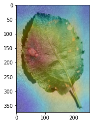
plt.imshow(superimposed_img)
plt.show()上で作成した関数を実際に使用して、判断根拠部位を可視化してみる。
gradcam(net_ft, '/path/to/image.jpg')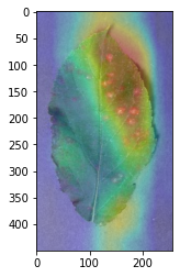
ResNet18
PyTorch で構築された(あるいは転移学習を行ったあとの) ResNet18 のモデルに Grad-CAM を適用する例を示す。モデルの訓練から Grad-CAM による可視化までコードは ![]() を参照。ここでは、すでに訓練済みのモデル
を参照。ここでは、すでに訓練済みのモデル net_ft が用意できた状態からの例を示す。まず、nent_ft を出力して、各層の構造を確認する。
print(net_ft)
# ResNet(
#   (conv1): Conv2d(3, 64, kernel_size=(7, 7), stride=(2, 2), padding=(3, 3), bias=False)
#   (bn1): BatchNorm2d(64, eps=1e-05, momentum=0.1, affine=True, track_running_stats=True)
#   (relu): ReLU(inplace=True)
#   (maxpool): MaxPool2d(kernel_size=3, stride=2, padding=1, dilation=1, ceil_mode=False)
#   (layer1): Sequential(
#     (0): BasicBlock(
#       (conv1): Conv2d(64, 64, kernel_size=(3, 3), stride=(1, 1), padding=(1, 1), bias=False)
#       (bn1): BatchNorm2d(64, eps=1e-05, momentum=0.1, affine=True, track_running_stats=True)
#       (relu): ReLU(inplace=True)
#       (conv2): Conv2d(64, 64, kernel_size=(3, 3), stride=(1, 1), padding=(1, 1), bias=False)
#       (bn2): BatchNorm2d(64, eps=1e-05, momentum=0.1, affine=True, track_running_stats=True)
#     )
#     (1): BasicBlock(
#       (conv1): Conv2d(64, 64, kernel_size=(3, 3), stride=(1, 1), padding=(1, 1), bias=False)
#       (bn1): BatchNorm2d(64, eps=1e-05, momentum=0.1, affine=True, track_running_stats=True)
#       (relu): ReLU(inplace=True)
#       (conv2): Conv2d(64, 64, kernel_size=(3, 3), stride=(1, 1), padding=(1, 1), bias=False)
#       (bn2): BatchNorm2d(64, eps=1e-05, momentum=0.1, affine=True, track_running_stats=True)
#     )
#   )
#   (layer2): Sequential(
#     (0): BasicBlock(
#       (conv1): Conv2d(64, 128, kernel_size=(3, 3), stride=(2, 2), padding=(1, 1), bias=False)
#       (bn1): BatchNorm2d(128, eps=1e-05, momentum=0.1, affine=True, track_running_stats=True)
#       (relu): ReLU(inplace=True)
#       (conv2): Conv2d(128, 128, kernel_size=(3, 3), stride=(1, 1), padding=(1, 1), bias=False)
#       (bn2): BatchNorm2d(128, eps=1e-05, momentum=0.1, affine=True, track_running_stats=True)
#       (downsample): Sequential(
#         (0): Conv2d(64, 128, kernel_size=(1, 1), stride=(2, 2), bias=False)
#         (1): BatchNorm2d(128, eps=1e-05, momentum=0.1, affine=True, track_running_stats=True)
#       )
#     )
#     (1): BasicBlock(
#       (conv1): Conv2d(128, 128, kernel_size=(3, 3), stride=(1, 1), padding=(1, 1), bias=False)
#       (bn1): BatchNorm2d(128, eps=1e-05, momentum=0.1, affine=True, track_running_stats=True)
#       (relu): ReLU(inplace=True)
#       (conv2): Conv2d(128, 128, kernel_size=(3, 3), stride=(1, 1), padding=(1, 1), bias=False)
#       (bn2): BatchNorm2d(128, eps=1e-05, momentum=0.1, affine=True, track_running_stats=True)
#     )
#   )
#   (layer3): Sequential(
#     (0): BasicBlock(
#       (conv1): Conv2d(128, 256, kernel_size=(3, 3), stride=(2, 2), padding=(1, 1), bias=False)
#       (bn1): BatchNorm2d(256, eps=1e-05, momentum=0.1, affine=True, track_running_stats=True)
#       (relu): ReLU(inplace=True)
#       (conv2): Conv2d(256, 256, kernel_size=(3, 3), stride=(1, 1), padding=(1, 1), bias=False)
#       (bn2): BatchNorm2d(256, eps=1e-05, momentum=0.1, affine=True, track_running_stats=True)
#       (downsample): Sequential(
#         (0): Conv2d(128, 256, kernel_size=(1, 1), stride=(2, 2), bias=False)
#         (1): BatchNorm2d(256, eps=1e-05, momentum=0.1, affine=True, track_running_stats=True)
#       )
#     )
#     (1): BasicBlock(
#       (conv1): Conv2d(256, 256, kernel_size=(3, 3), stride=(1, 1), padding=(1, 1), bias=False)
#       (bn1): BatchNorm2d(256, eps=1e-05, momentum=0.1, affine=True, track_running_stats=True)
#       (relu): ReLU(inplace=True)
#       (conv2): Conv2d(256, 256, kernel_size=(3, 3), stride=(1, 1), padding=(1, 1), bias=False)
#       (bn2): BatchNorm2d(256, eps=1e-05, momentum=0.1, affine=True, track_running_stats=True)
#     )
#   )
#   (layer4): Sequential(
#     (0): BasicBlock(
#       (conv1): Conv2d(256, 512, kernel_size=(3, 3), stride=(2, 2), padding=(1, 1), bias=False)
#       (bn1): BatchNorm2d(512, eps=1e-05, momentum=0.1, affine=True, track_running_stats=True)
#       (relu): ReLU(inplace=True)
#       (conv2): Conv2d(512, 512, kernel_size=(3, 3), stride=(1, 1), padding=(1, 1), bias=False)
#       (bn2): BatchNorm2d(512, eps=1e-05, momentum=0.1, affine=True, track_running_stats=True)
#       (downsample): Sequential(
#         (0): Conv2d(256, 512, kernel_size=(1, 1), stride=(2, 2), bias=False)
#         (1): BatchNorm2d(512, eps=1e-05, momentum=0.1, affine=True, track_running_stats=True)
#       )
#     )
#     (1): BasicBlock(
#       (conv1): Conv2d(512, 512, kernel_size=(3, 3), stride=(1, 1), padding=(1, 1), bias=False)
#       (bn1): BatchNorm2d(512, eps=1e-05, momentum=0.1, affine=True, track_running_stats=True)
#       (relu): ReLU(inplace=True)
#       (conv2): Conv2d(512, 512, kernel_size=(3, 3), stride=(1, 1), padding=(1, 1), bias=False)
#       (bn2): BatchNorm2d(512, eps=1e-05, momentum=0.1, affine=True, track_running_stats=True)
#     )
#   )
#   (avgpool): AdaptiveAvgPool2d(output_size=(1, 1))
#   (fc): Linear(in_features=512, out_features=5, bias=True)
# )
ResNet18 は、residue block とよばれるモジュールが複数重ねられて作られたアーキテクチャである。そのため、ResNet18 のアーキテクチャは、畳み込み層やプーリング層を単純に重ねただけの VGG16 よりも複雑に見える。
ResNet18 のモジュールを確認すると、conv1、bn1、relu、maxpool、layer1、layer2、layer3、layer4、avgpool、fc のように並んでいる。最後の畳み込み層の出力は、layer4 の出力値である。そこで、ResNet18 モデルに画像を代入して、layer4 モジュールまでいったん実行して、その出力値を変数に保存する。その後に、layer4 モジュールの出力値を avgpool および fc モジュールに代入して、予測結果を得る。最後に、layer4 モジュールの出力値と予測結果から Grad-CAM を計算して可視化する。
可視化関数は、画像を代入するときのモデルのモジュール名が異なっていることを除けば、基本的に VGG16 のときの関数と全く同じである。
def gradcam(net, img_fpath):

    net.eval()

    def __extract(grad):
        global feature_grad
        feature_grad = grad

    img = PIL.Image.open(img_fpath).convert('RGB')
    transforms = torchvision.transforms.Compose([
        torchvision.transforms.Resize(256),
        torchvision.transforms.CenterCrop(224),
        torchvision.transforms.ToTensor(),
        torchvision.transforms.Normalize([0.485, 0.456, 0.406], [0.229, 0.224, 0.225])
    ])

    img = transforms(img)
    img = img.unsqueeze(0)

    # get features from the last convolutional layer
    x = net.conv1(img)
    x = net.bn1(x)
    x = net.relu(x)
    x = net.maxpool(x)
    x = net.layer1(x)
    x = net.layer2(x)
    x = net.layer3(x)
    x = net.layer4(x)
    features = x

    # hook for the gradients
    def __extract_grad(grad):
        global feature_grad
        feature_grad = grad
    features.register_hook(__extract_grad)

    # get the output from the whole VGG architecture
    x = net.avgpool(x)
    x = x.view(x.size(0), -1)
    output = net.fc(x)
    pred = torch.argmax(output).item()
    print(pred)

    # get the gradient of the output
    output[:, pred].backward()

    # pool the gradients across the channels
    pooled_grad = torch.mean(feature_grad, dim=[0, 2, 3])

    # weight the channels with the corresponding gradients
    # (L_Grad-CAM = alpha * A)
    features = features.detach()
    for i in range(features.shape[1]):
        features[:, i, :, :] *= pooled_grad[i]

    # average the channels and create an heatmap
    # ReLU(L_Grad-CAM)
    heatmap = torch.mean(features, dim=1).squeeze()
    heatmap = np.maximum(heatmap, 0)

    # normalization for plotting
    heatmap = heatmap / torch.max(heatmap)
    heatmap = heatmap.numpy()

    # project heatmap onto the input image
    img = cv2.imread(img_fpath)
    heatmap = cv2.resize(heatmap, (img.shape[1], img.shape[0]))
    heatmap = np.uint8(255 * heatmap)
    heatmap = cv2.applyColorMap(heatmap, cv2.COLORMAP_JET)
    superimposed_img = heatmap * 0.4 + img
    superimposed_img = np.uint8(255 * superimposed_img / np.max(superimposed_img))
    superimposed_img = cv2.cvtColor(superimposed_img, cv2.COLOR_BGR2RGB)
    plt.imshow(superimposed_img)
    plt.show()
上で作成した関数を実際に使用して、判断根拠部位を可視化してみる。
gradcam(net_ft, '/path/to/image.jpg')